Bayesian Optimization of UV Curable Elastomer
Introduction
Let's use Bayesian optimization to efficiently design a UV curable elastomer. Note for this post I'll use a mix of real and synthetic data for illustrative purposes.
If you're not familiar with the concept of Bayesian optimization and how it compares to OFAT and DOE, check out: https://en.wikipedia.org/wiki/Bayesian_optimization, https://distill.pub/2020/bayesian-optimization/
High Level Comparison
| OFAT | DOE | Bayesian Optimization | |
|---|---|---|---|
| Approach | Change one factor at a time to understand impact on dependent variable / output, eg: Raw Material X loading vs material Tg | Systematic method to understanding relationships between multiple factors or variables and key outputs of interest, eg: changing loading of Raw Material X and Raw Material Y vs material Tg | Black-box optimization, experiments are generated and tested in batches, each batch result is used to guide next set of experiments |
| Number of experiments | Large | Moderate | Least |
| Account for interactions between factors | No | Yes | Yes |
| Active Learning | No | No | Yes |
| Ideal for | Quick screening, optimizing simple systems with very limited interactions, provide starting points for DOE | Interactions between factors must be well understood, able to run many experiments for optimizing | Optimizing where experimentation is costly or time consuming |
There are several open and closed source options for performing Bayesian optimization, for this post I'll be using BayBE (https://emdgroup.github.io/baybe/stable/index.html)
The maintainers have a good intro video here:
https://www.youtube.com/watch?v=EcVvYhh4wI0&t=1258s&pp=ygUMYmF5YmUgcHl0aG9u
Installation
I recommend installing BayBE with chem and insights modules (can leverage molecular descriptors and fingerprints in model during optimization from chem module, Shapley values from insights module, save for another post)
pip install baybe[chem,insights]
I'll also be using RDKit for some early screening, but not needed.
pip install rdkit
Targets
As an example, we will design a UV-curable elastomer targeting the properties outlined below. Note this is intended for demonstrative purposes only and does not represent a complete formulation or an exhaustive list of physical and mechanical property requirements.
| Property | Value | Standard |
|---|---|---|
| Ultimate Tensile Strength | >= 10 MPa | ASTM D412 |
| Resilience | >= 50% | Internal Method |
| Viscosity | <= 1750 cP @ 25C | ASTM D7867 |
Table 1: Key Properties
Raw materials:
- 9 monomers (Tg, SMILES known)
- Oligomer_1 (Polyurethane methacrylate elastomer, high viscosity)
- Oligomer_2 (Polyurethane methacrylate elastomer, medium viscosity)
- Oligomer_3 (Polyurethane methacrylate elastomer, low viscosity)
Prescreening
Operating under the following assumptions:
- High Tg monomers needed to impart strength but will worsen resilience / energy return
- Higher viscosity oligomers potentially higher molecular weight, possibly higher resilience, but lower crosslink density and strength
I'll start with a theory that while bulky steric groups impart strength they will also reduce resilience of the cured elastomer, loss modulus will increase (think rubber-band snapping back), thus need to find good trade-off between Tg and bulkiness in monomers. For this I'll use RDKit to calculate van der waals volume for each monomer based on its SMILES string then divide its literature Tg by calculated volume.
from rdkit import Chem
from rdkit.Chem import AllChem
import pandas as pd

def get_vdw_volume(smiles: str) -> float:
    mol = Chem.MolFromSmiles(smiles)
    mol = Chem.AddHs(mol)
    AllChem.EmbedMolecule(mol)
    AllChem.MMFFOptimizeMolecule(mol)
    vdw_volume = AllChem.ComputeMolVolume(mol) # A^3
    return vdw_volume

high_tg_monomers = pd.DataFrame(
    {
        "monomers": [
            "IBOMA",
            "Monomer D",
            "Monomer C",
            "Monomer B",
            "Monomer A",
            "HEMA",
            "tert-Butyl methacrylate",
            "Neopentyl methacrylate",
        ],
        "smiles": [
            "CC(=C)C(=O)OC1CC2CCC1(C)C2(C)C",
            "CC1(C)[C@H]2CC[C@]1(C)[C@H](C2)OC(=O)C=C",
            "CC1(C)[C@H]2CC[C@]1(C)[C@H](C2)OC(=O)C=C",
            "CC1(C)[C@H]2CC[C@]1(C)[C@H](C2)OC(=O)C=C",
            "CC1(C)[C@H]2CC[C@]1(C)[C@H](C2)OC(=O)C=C",
            "CC1(C)[C@H]2CC[C@]1(C)[C@H](C2)OC(=O)C=C",
            "CC(=C)C(=O)OCCO",
            "CC(=C)C(=O)OC(C)(C)C",
            "CC(=C)C(=O)OCC(C)(C)C",
        ],
        "Tg": [115, 125, 145, 142, 147, 175, 55, 107, 110],
    }
)

vdw = []
for i in high_tg_monomers["smiles"]:
    vdw.append(get_vdw_volume(i))
high_tg_monomers["vdw_volume"] = vdw
high_tg_monomers["Tg/vdw_volume"] = high_tg_monomers["Tg"] / high_tg_monomers["vdw_volume"]
print(high_tg_monomers.sort_values("Tg/vdw_volume", ascending=False).to_string())
Which gives us:
| monomers | smiles | Tg | vdw_volume | Tg/vdw_volume |
| Monomer C | 145 | 136.57600000000002 | 1.0616799437675724 | |
| Monomer B | 147 | 143.48000000000005 | 1.0245330359632001 | |
| Monomer D | 142 | 151.27200000000005 | 0.9387064360886347 | |
| Monomer A | 175 | 162.37600000000003 | 0.8252451101147951 | |
| tert-Butyl methacrylate | CC(=C)C(=O)OC(C)(C)C | 107 | 151.51200000000003 | 0.7062146892655365 |
| Neopentyl methacrylate | CC(=C)C(=O)OCC(C)(C)C | 110 | 168.61600000000004 | 0.6523698818617448 |
| IBOMA | CC(=C)C(=O)OC1CC2CCC1(C)C2(C)C | 115 | 230.83200000000005 | 0.4981978235253343 |
| HEMA | CC(=C)C(=O)OCCO | 55 | 127.28800000000003 | 0.4320910062221104 |
We'll filter out monomers with lower Tg/vdw ratios to reduce search space with the exception of IBOMA as we expect it to perform poorly (will our theory hold water...).
Bayesian Optimization
The Setup
In order to perform Bayesian optimization we must set the following:
- Targets / objectives
- Selecting multi-objective for: UTS, resilience, viscosity
- Objective type
- Selecting Pareto Objective (This approach allows one to select the optimal trade-offs in target properties after optimization has been completed. An alternative is to combine objectives into a single scoring function using user-defined weights. However, the later approach (DesirabilityObjective) requires those weights to be specified before optimization, meaning that if the relative importance of the objectives or target properties changes, the optimization must be rerun)
- Search space
- Individual monomers may be included between 0-50% by wt.
- Individual oligomers may be included between 0-60% by wt.
- Total monomer content must be between 20-50% by wt.
- The above bounds and constraints are based on prior knowledge / screening, monomer loadings below threshold are not likely to exhibit adequate strength, monomer loadings above threshold are likely to restrict too much movement
- Combined monomer and oligomer content must sum to 100% by wt.
- Recommended formulations must have raw material cost below $26/kg
- Recommender
- We initially start with randomly sampling the search space to get first set of recommendations then switch to Bayesian optimization via BotorchRecommender
We instantiate the Campaign class with the specified parameters and generate the initial set of recommended formulations. Because optimization is an iterative process, requiring formulations to be physically tested, resulting data fed back into the system, and new recommendations generated, the campaign state and recommendations must persist throughout the experiment cycle. Thus we serialize the campaign object to a JSON file while the recommended formulations are exported to a CSV file. This allows experiment data to be collected and subsequently reintroduced into the optimization process across iterations.
create_campaign.py
import json
from baybe.targets import NumericalTarget
from baybe.objectives import ParetoObjective
from baybe.parameters import NumericalContinuousParameter
from baybe.searchspace import SearchSpace
from baybe.constraints import ContinuousLinearConstraint
from baybe.recommenders import (
    BotorchRecommender,
    TwoPhaseMetaRecommender,
    RandomRecommender,
)
from baybe import Campaign

try:
    with open("campaign.json", "r", encoding="utf-8") as file:
        campaign = Campaign.from_json(str(json.load(file)))
    print("Campaign already exists")
except:
    target_1 = NumericalTarget(name="UTS")
	target_2 = NumericalTarget(name="resilience")
    target_3 = NumericalTarget.match_absolute(
        name="viscosity", match_value=17500, match_mode="<="
    )
    objective = ParetoObjective(
        targets=[target_1, target_2, target_3]
    )

    parameters = [
        NumericalContinuousParameter(name="Monomer_A", bounds=(0, 0.5)),
        NumericalContinuousParameter(name="Monomer_B", bounds=(0, 0.5)),
        NumericalContinuousParameter(name="Monomer_C", bounds=(0, 0.5)),
        NumericalContinuousParameter(name="Monomer_D", bounds=(0, 0.5)),
        NumericalContinuousParameter(name="IBOMA", bounds=(0, 0.5)),
        NumericalContinuousParameter(name="Oligomer_1", bounds=(0, 0.6)),
        NumericalContinuousParameter(name="Oligomer_2", bounds=(0, 0.6)),
        NumericalContinuousParameter(name="Oligomer_3", bounds=(0, 0.6)),
    ]

    constraints = [
        ContinuousLinearConstraint(
            parameters=[
                "Monomer_A",
                "Monomer_B",
                "Monomer_C",
                "Monomer_D",
                "IBOMA",
                "Oligomer_1",
                "Oligomer_2",
                "Oligomer_3",
            ],
            operator="=",
            coefficients=(1.0, 1.0, 1.0, 1.0, 1.0, 1.0, 1.0, 1.0),
            rhs=1.0,  # All components must sum to 100%
        ),
        ContinuousLinearConstraint(
            parameters=["Monomer_A", "Monomer_B", "Monomer_C", "Monomer_D", "IBOMA"],
            operator="<=",
            coefficients=(1.0, 1.0, 1.0, 1.0, 1.0),
            rhs=0.5,  # Total monomer loading must be less than or equal to 50%
        ),
        ContinuousLinearConstraint(
            parameters=["Monomer_A", "Monomer_B", "Monomer_C", "Monomer_D", "IBOMA"],
            operator=">=",
            coefficients=(1.0, 1.0, 1.0, 1.0, 1.0),
            rhs=0.2,  # Total monomer loading must be greater than or equal to 20%
        ),
        ContinuousLinearConstraint(
            parameters=[
                "Monomer_A",
                "Monomer_B",
                "Monomer_C",
                "Monomer_D",
                "IBOMA",
                "Oligomer_1",
                "Oligomer_2",
                "Oligomer_3",
            ],
            operator="<=",
            coefficients=(
                25,
                14,
                32,
                17,
                23,
                24,
                20,
                23,
            ),  # Each coefficient represents raw material cost $/kg
            rhs=2600,  # Total raw cost must be less than or equal to $26/kg
        ),
    ]

    searchspace = SearchSpace.from_product(
        parameters=parameters, constraints=constraints
    )

    recommender = TwoPhaseMetaRecommender(
        initial_recommender=RandomRecommender(),
        recommender=BotorchRecommender(),
    )

    campaign = Campaign(searchspace, objective, recommender)
    recommended_experiments = campaign.recommend(batch_size=3)

    with open("campaign.json", "w") as file:
        json.dump(campaign.to_json(), file)

    for i in range(0, len(campaign.targets)):
        recommended_experiments[campaign.targets[i].to_dict()["name"]] = ""
    recommended_experiments.to_csv("recommended_experiments.csv")

    print("Created campaign, wrote to campaign.json")
    print("Created initial recommendations, wrote to recommended_experiments.csv")
recommended_experiments.csv
| Monomer_A | Monomer_B | Monomer_C | Monomer_D | IBOMA | Oligomer_1 | Oligomer_2 | Oligomer_3 | |
| 0 | 0.080585 | 0.060319 | 0.026637 | 0.043217 | 0.053373 | 0.041021 | 0.126362 | 0.568485 |
| 1 | 0.054061 | 0.049533 | 0.06048 | 0.094934 | 0.041493 | 0.153746 | 0.002766 | 0.542986 |
| 2 | 0.121567 | 0.124872 | 0.149433 | 0.009767 | 0.057253 | 0.263017 | 0.031103 | 0.242988 |
Go in the lab, test formulations, update CSV with results:
| Monomer_A | Monomer_B | Monomer_C | Monomer_D | IBOMA | Oligomer_1 | Oligomer_2 | Oligomer_3 | UTS | resilience | viscosity | |
| 0 | 0.080585 | 0.060319 | 0.026637 | 0.043217 | 0.053373 | 0.041021 | 0.126362 | 0.568485 | 7.932372 | 50.74958 | 14012.43 |
| 1 | 0.054061 | 0.049533 | 0.06048 | 0.094934 | 0.041493 | 0.153746 | 0.002766 | 0.542986 | 8.479434 | 47.47501 | 14191.44 |
| 2 | 0.121567 | 0.124872 | 0.149433 | 0.009767 | 0.057253 | 0.263017 | 0.031103 | 0.242988 | 10.47866 | 19.16858 | 14739.55 |
Now we'd like to update our campaign with test results:
update_campaign.py
import json
from baybe import Campaign
import numpy as np
import pandas as pd

try:
    with open("campaign.json", "r", encoding="utf-8") as file:
        campaign = Campaign.from_json(str(json.load(file)))
    print("Loaded campaign...")
except:
    raise ValueError("Campaign does not exist")

try:
    recommended_experiments = pd.read_csv("recommended_experiments.csv")
    recommended_experiments = recommended_experiments.reset_index(drop=True)
    recommended_experiments = recommended_experiments.replace("", np.nan).dropna()

    filter = campaign.measurements.filter(regex=r"^(?!.*BatchNr)").filter(
        regex=r"^(?!.*FitNr)"
    )
    new_measurements_only = pd.concat(
        [filter, recommended_experiments]
    ).drop_duplicates(keep=False)

    if not new_measurements_only.empty:
        print(
            "New measurements imported from recommended_experiments.csv and added to campaign"
        )
        campaign.add_measurements(new_measurements_only)
        with open("campaign.json", "w") as file:
            json.dump(campaign.to_json(), file)
        print("Updated campaign.json")
    else:
        print("No new measurements in recommended_experiments.csv, doing nothing")

except:
    print("No recommended_experiments.csv to update from")
- This will only import test results for formulations that contain data for every target, missing data will cause entire formulation row to be skipped
Now we perform Bayesian optimization with initial results, recommend next batch of formulations to test, and update both campaign.json and recommended_experiments.csv files:
recommend_formulations.py
import json
from baybe import Campaign

try:
    with open("campaign.json", "r", encoding="utf-8") as file:
        campaign = Campaign.from_json(str(json.load(file)))
    print("Loaded campaign...")
except:
    raise ValueError("Campaign does not exist")

recommended_experiments = campaign.recommend(batch_size=3)

for i in range(0, len(campaign.targets)):
    recommended_experiments[campaign.targets[i].to_dict()["name"]] = ""

recommended_experiments.to_csv("recommended_experiments.csv", mode="a", header=False)
print("Added recommendations to recommended_experiments.csv")

with open("campaign.json", "w") as file:
    json.dump(campaign.to_json(), file)
print("Updated campaign.json")
Once the next batch of experimental data has been collected only update_campaign.py and recommend_formulations.py are required to continue the optimization process.
After multiple iterations of optimization we have the following formulations and collected properties:
| Monomer_A | Monomer_B | Monomer_C | Monomer_D | IBOMA | Oligomer_1 | Oligomer_2 | Oligomer_3 | UTS | resilience | viscosity | |
| 0 | 0.080585 | 0.060319 | 0.026637 | 0.043217 | 0.053373 | 0.041021 | 0.126362 | 0.568485 | 7.932372 | 50.74958 | 14012.43 |
| 1 | 0.054061 | 0.049533 | 0.06048 | 0.094934 | 0.041493 | 0.153746 | 0.002766 | 0.542986 | 8.479434 | 47.47501 | 14191.44 |
| 2 | 0.121567 | 0.124872 | 0.149433 | 0.009767 | 0.057253 | 0.263017 | 0.031103 | 0.242988 | 10.47866 | 19.16858 | 14739.55 |
| 3 | 0 | 0.000471 | 0.10914 | 0.090388 | 0 | 0.33288 | 0 | 0.46712 | 7.0473 | 74.6849 | 18184.9 |
| 4 | 5.90E-17 | 0.000433 | 0.109157 | 0.09041 | 7.30E-18 | 0.332847 | 4.49E-17 | 0.467153 | 7.04769 | 74.68382 | 18184.43 |
| 5 | 5.40E-15 | 0.030859 | 0.068278 | 0.100862 | 0 | 0.338996 | 0 | 0.461004 | 6.572938 | 75.45074 | 18129.23 |
| 6 | 5.49E-14 | 0.108457 | 0.155518 | 0.079058 | 0.046601 | 0.292629 | 0.076353 | 0.241384 | 9.731184 | 37.49173 | 16469.54 |
| 7 | 0.360422 | 0.05298 | 0.086598 | 1.65E-08 | 1.91E-09 | 0.232216 | 0.04021 | 0.227574 | 9.928362 | 14.41756 | 13660.7 |
| 8 | 6.88E-16 | 0.010919 | 0.105146 | 0.088812 | 1.98E-14 | 0.55543 | 2.27E-14 | 0.239693 | 6.07994 | 79.52812 | 21461.61 |
| 9 | 3.60E-13 | 9.79E-14 | 0.273934 | 3.34E-13 | 2.25E-13 | 0.270912 | 2.94E-11 | 0.455155 | 9.741209 | 58.83441 | 17146.14 |
| 10 | 0 | 0 | 0.188857 | 0.311143 | 0 | 0.192357 | 0 | 0.307643 | 12.13377 | 21.97606 | 12985.21 |
| 11 | 0 | 0 | 0.136588 | 4.57E-15 | 0.363412 | 0.219551 | 0 | 0.280449 | 12.44863 | 5.4377 | 12903.52 |
| 12 | 7.20E-16 | 1.05E-16 | 0.332646 | 0.167354 | 6.01E-16 | 0.151892 | 0.035608 | 0.3125 | 13.55733 | 19.44856 | 13381.37 |
| 13 | 0 | 0 | 0.263234 | 0 | 0 | 0.133182 | 0.206556 | 0.397029 | 9.756699 | 60.98161 | 17220.64 |
| 14 | 0 | 0 | 0.172798 | 0.327202 | 2.21E-15 | 0.115119 | 0.284309 | 0.100572 | 11.83952 | 25.40356 | 14597.46 |
| 15 | 8.68E-15 | 3.43E-15 | 0.3367 | 0.035911 | 1.19E-14 | 0.158319 | 0.113586 | 0.355483 | 11.84142 | 41.33415 | 15740.76 |
| 16 | 0 | 0 | 0.449295 | 0.050705 | 0 | 0.186906 | 0.176808 | 0.136285 | 14.22683 | 21.11579 | 15843.5 |
| 17 | 3.45E-15 | 1.16E-15 | 0.5 | 0 | 7.43E-15 | 0 | 0 | 0.5 | 15.8 | 12.5 | 11500 |
| 18 | 9.10E-11 | 0 | 0.5 | 1.94E-11 | 2.57E-10 | 3.04E-11 | 0.457213 | 0.042787 | 15.02274 | 20.72983 | 16072.13 |
| 19 | 0 | 0.5 | 1.40E-07 | 0 | 0 | 2.24E-23 | 0.5 | 0 | 9.150001 | 29 | 14850 |
| 20 | 0 | 0 | 0.2 | 0 | 0 | 1.10E-14 | 0.555966 | 0.244034 | 8.374858 | 75.00739 | 19159.66 |
| 21 | 0 | 0 | 0.398611 | 3.49E-12 | 0 | 0 | 0.400485 | 0.200905 | 12.92917 | 37.45182 | 16214.57 |
| 22 | 1.92E-12 | 4.01E-12 | 0.326238 | 2.66E-12 | 4.29E-11 | 1.47E-12 | 0.422477 | 0.251285 | 11.32853 | 50.51296 | 16941.1 |
| 23 | 5.08E-14 | 3.84E-14 | 0.2 | 5.56E-14 | 3.16E-13 | 0.259794 | 0.540206 | 0 | 7.274143 | 81.21856 | 22898.97 |
| 24 | 0 | 0.051102 | 0.148898 | 0 | 0 | 0 | 0.376408 | 0.423592 | 8.087323 | 72.54188 | 17195.45 |
| 25 | 0 | 7.84E-14 | 0.405818 | 0 | 0.094182 | 0 | 0 | 0.5 | 15.1784 | 0.727292 | 11010.26 |
| 26 | 0 | 0 | 0.45176 | 9.71E-11 | 2.69E-11 | 2.92E-10 | 0.508056 | 0.040184 | 13.89432 | 30.087 | 16918.24 |
| 27 | 0.029485 | 0.017142 | 0.117793 | 0.03558 | 1.25E-11 | 0.099973 | 0.411155 | 0.288872 | 7.322505 | 75.24868 | 18867.68 |
| 28 | 0 | 0.134232 | 0.30128 | 3.92E-11 | 5.92E-11 | 0 | 0.564488 | 2.77E-11 | 11.89034 | 35.95959 | 17153.32 |
| 29 | 0.075858 | 0 | 0 | 0.124142 | 0 | 0 | 0.525032 | 0.274968 | 6.417801 | 75.17485 | 17965.5 |
| 30 | 6.62E-24 | 0 | 0.227325 | 2.07E-23 | 8.45E-24 | 0 | 0.413894 | 0.358782 | 9.20659 | 67.6683 | 17547.67 |
| 31 | 0 | 0 | 0.5 | 3.58E-24 | 4.52E-25 | 0 | 0.245289 | 0.254711 | 15.38301 | 16.91521 | 13952.89 |
| 32 | 0 | 0 | 0.4 | 0 | 0 | 0 | 0.6 | 0 | 12.62 | 40.8 | 18200 |
ID11 tested with 36% IBOMA loading resulted in ~5% resilience and causes IBOMA to primarily be avoided in future tests.
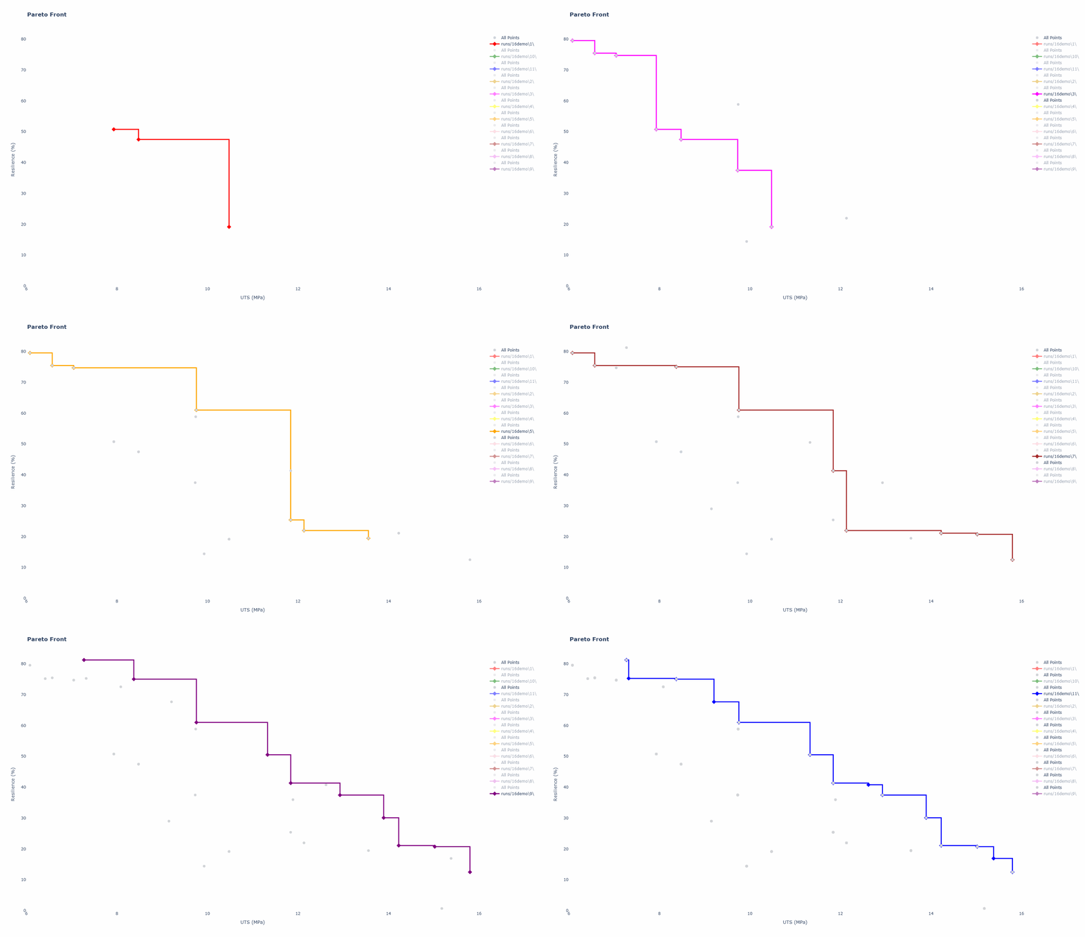
Since we selected Pareto Objective we end up with a set of optimal compromises where we can seek out a formulation matching our original targets, eg: ID22, but we also have access to other formulations that may be of interest, eg: if product requirements shift mid project perhaps ID20 with a lower UTS and higher resilience value addresses our updated needs:
| ID | Monomer_A | Monomer_B | Monomer_C | Monomer_D | Monomer_E | Oligomer_1 | Oligomer_2 | Oligomer_3 | UTS | resilience | viscosity |
|---|---|---|---|---|---|---|---|---|---|---|---|
| 13 | 0 | 0 | 0.263234 | 0 | 0 | 0.133182 | 0.206556 | 0.397029 | 9.756699 | 60.98161 | 17220.64 |
| 20 | 0 | 0 | 0.2 | 0 | 0 | 0.0000 | 0.555966 | 0.244034 | 8.374858 | 75.00739 | 19159.66 |
| 22 | 0.0000 | 0.0000 | 0.3262 | 0.0000 | 0.0000 | 0.0000 | 0.422477 | 0.251285 | 11.32853 | 50.51296 | 16941.1 |
Pareto Front of UTS vs Resilience for each optimization cycle:
I'll end with a few points for consideration:
Bayesian optimization becomes increasingly challenging to leverage as the number of objectives grows, eg: 4, 5, 6... Each additional objective generally requires its own surrogate model, increasing computational cost and model complexity. At the same time, the size of the Pareto front typically grows with the number of objectives, creating a larger set of potentially optimal trade-offs. This makes it more difficult to efficiently explore the design space, distinguish meaningful improvements between candidates, and achieve convergence.
BayBE offers a broad range of capabilities, and its documentation is well worth reviewing. Two features that are particularly noteworthy:
- Transfer learning allows existing experimental data and prior learnings from previous campaigns to be used in new campaigns and ultimately accelerate optimization
- Molecular descriptors can also be incorporated as parameter representations, either by supplying SMILES strings and selecting Scikit-fingerprint fingerprint type, or through custom descriptor dictionaries, eg: including Tg, MW, etc. Incorporating these descriptors provides the model with chemically meaningful information and can improve predictions compared with relying solely on categorical material labels--such incorporation does however increase dimensionality and require more compute.